Beyond Last-Click: How to Measure True User Retention in GA4 with BigQuery

In the world of e-commerce, where every click and conversion is critical, we often focus on immediate metrics like CPA or ROAS. We want to know which campaign brought the last click. But what about the long-term customer value? Could a campaign that costs more today turn out to be a goldmine tomorrow because it acquires the most loyal customers?

The answer lies in cohort analysis. It's a powerful tool that allows us to look at groups of users over time and see how they behave after acquisition. This way, we can discover which marketing campaigns, sources, and channels attract customers who return and make repeat purchases.

While Google Analytics 4 offers basic retention reports, the full freedom of analysis lies in BigQuery. Our team, leveraging this platform, has developed a complete SQL query that enables detailed retention analysis segmented by campaign, source, and week.

How Our SQL Query for Cohort Analysis Works

Here's a breakdown of what our script does (which you can use in your own project), split into 7 logical steps:

1. Cohort Identification: The script starts by finding all users who had their "first_visit" within a selected period (e.g., January 2025). This creates precise cohorts that will form the basis of our analysis.
2. Size Determination: We count how many users are in each of these cohorts. This is our starting point.
3. Purchase Search: Next, we scan our entire database for "purchase" events that occurred within our chosen retention period (e.g., until March 31, 2025).
4. Data Linking: We join the first-visit data with the purchase data. This allows us to calculate how many weeks have passed between a user's acquisition and their purchase.
5. Buyer Count: We count the number of unique users who made a purchase in each subsequent week after acquisition.
6. Pivot: This part of the script transforms rows of data into a readable table with columns for each week of retention (e.g., "week_0," "week_1," etc.).
7. Final Output: The final query combines all the data to deliver a complete report. We get the number of buyers in each week and the key metric: the retention rate, which is the percentage of users from a given cohort who returned in subsequent weeks to make a purchase.

‍

‍

SQL Output

The SQL presented below returns a simple table:

‍

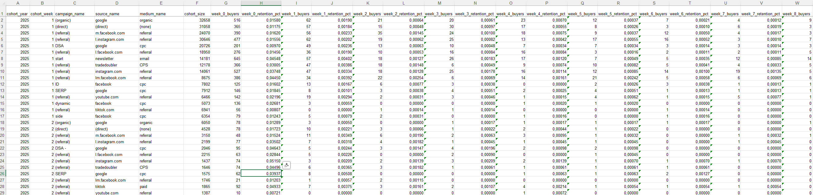
In the next steps, you can build a fully automated dashboard in any BI tool and simply pass the link to the appropriate stakeholders.

‍

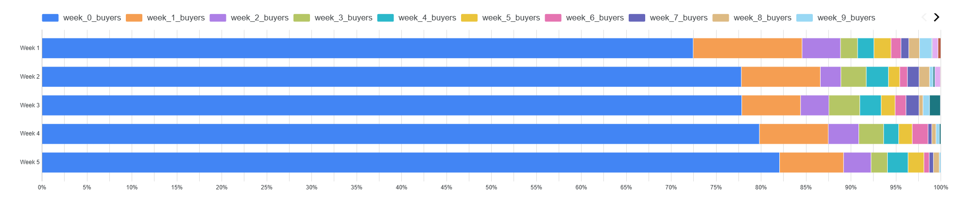
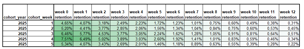
Or create a custom visualisation in Excel ad hoc (we know well that you can't live without Excel :))

‍

What This Means for Your Marketing Strategy

With a report like this, you stop guessing. You'll discover which channels (e.g., email marketing, Facebook ads, Google Ads) not only attract users but also build lasting relationships that lead to repeat conversions.

You can make strategic decisions by shifting budget from campaigns that generate "one-time" customers to those that build a loyal base.

Want to learn more about retention analysis or need help with its implementation?

At Defused Data, cohort analysis is our forte. We see enormous potential in this approach, and this post aims to promote it. Why do we think it's a must-have for every business?

1. The data is practically available at your fingertips (and thanks to our query, you no longer have the excuse of not knowing how to access it) and doesn't require any special GA4 configuration—it's simply there, so it's a shame not to use it.
2. Cohorts allow you to elevate your analyses to the next level and surprise business owners (positively). You can stop relying solely on conversion rates and show management how your campaigns are impacting the business over a longer timeframe.

‍

Here is the query ready to use:

Below, we will go through the SQL code step by step:

1. Configuration

This code block sets up variables, making it easy to change the date ranges for your analysis without editing the rest of the query.

DECLARE cohort_start DATE;
DECLARE cohort_end DATE;
DECLARE sales_end DATE;

SET cohort_start = '2025-01-01';
SET cohort_end   = '2025-01-31';
SET sales_end    = '2025-03-31';

‍

2. CohortUsers

This block identifies unique users who had their first visit within the specified time window. This is the crucial step that creates cohorts based on the acquisition date and campaign.

WITH CohortUsers AS (
  SELECT
    user_pseudo_id,
    DATE(MIN(TIMESTAMP_MICROS(event_timestamp))) AS first_visit_date,
    EXTRACT(ISOYEAR FROM MIN(TIMESTAMP_MICROS(event_timestamp))) AS cohort_year,
    EXTRACT(ISOWEEK FROM MIN(TIMESTAMP_MICROS(event_timestamp))) AS cohort_week,
    COALESCE(traffic_source.name,
             (SELECT value.string_value FROM UNNEST(event_params) WHERE key = 'campaign')) AS campaign_name,
    COALESCE(traffic_source.source,
             (SELECT value.string_value FROM UNNEST(event_params) WHERE key = 'source'))   AS source_name,
    COALESCE(traffic_source.medium,
             (SELECT value.string_value FROM UNNEST(event_params) WHERE key = 'medium'))   AS medium_name
  FROM  `your-project-id.analytics_123456789.events_*`
  WHERE _TABLE_SUFFIX BETWEEN FORMAT_DATE('%Y%m%d', cohort_start) AND FORMAT_DATE('%Y%m%d', cohort_end)
    AND event_name = 'first_visit'
    AND user_pseudo_id IS NOT NULL
  GROUP BY user_pseudo_id, campaign_name, source_name, medium_name
)

Description:

• It selects first_visit events within the defined range.
• MIN(TIMESTAMP_MICROS(event_timestamp)) determines the exact date of a user's first visit, and EXTRACT on ISO-year and ISO-week creates unique identifiers for each cohort.
• COALESCE prioritises traffic source fields for campaign data. If a field is empty, the query falls back to the event_params.

‍

3.  CohortSize

This block counts how many unique users are in each defined cohort. This is essential for calculating the retention rate.

CohortSize AS (
  SELECT
    cohort_year, cohort_week, campaign_name, source_name, medium_name,
    COUNT(DISTINCT user_pseudo_id) AS cohort_size
  FROM CohortUsers
  GROUP BY cohort_year, cohort_week, campaign_name, source_name, medium_name
)

Description:

• It groups the data from the CohortUsers table by (cohort_year, cohort_week, campaign_name, source_name, medium_name).
• COUNT(DISTINCT user_pseudo_id) counts the unique users in each group.

‍

4. UserSales

This block aggregates the purchase value for each user on a daily basis.

UserSales AS (
  SELECT
    user_pseudo_id,
    DATE(TIMESTAMP_MICROS(event_timestamp)) AS purchase_date,
    SUM(
        (SELECT value.double_value FROM UNNEST(event_params) WHERE key = 'value')
    ) AS purchase_value
  FROM  `your-project-id.analytics_123456789.events_*`
  WHERE event_name = 'purchase'
    AND _TABLE_SUFFIX BETWEEN FORMAT_DATE('%Y%m%d', cohort_start) AND FORMAT_DATE('%Y%m%d', sales_end)
  GROUP BY user_pseudo_id, purchase_date
)

Description:

• It selects all purchase events within a wider date range (from cohort_start to sales_end), allowing it to capture purchases that occurred after the acquisition date.
• SUM((SELECT value.double_value FROM UNNEST(event_params) WHERE key = 'value')) sums the value of all purchases made by a user on a single day.

‍

5.  CohortSales

CohortSales AS (
  SELECT
    cu.cohort_year, cu.cohort_week, cu.campaign_name, cu.source_name, cu.medium_name,
    DATE_DIFF(
      DATE_TRUNC(us.purchase_date, WEEK(MONDAY)),
      DATE_TRUNC(cu.first_visit_date, WEEK(MONDAY)),
      WEEK
    ) AS weeks_since_acquisition,
    cu.user_pseudo_id
  FROM CohortUsers cu
  LEFT JOIN UserSales us
    ON cu.user_pseudo_id = us.user_pseudo_id
   AND DATE_DIFF(
         DATE_TRUNC(us.purchase_date, WEEK(MONDAY)),
         DATE_TRUNC(cu.first_visit_date, WEEK(MONDAY)),
         WEEK
       ) >= 0
)

Description:

• LEFT JOIN on user_pseudo_id is crucial to keep all users from the cohorts, even if they haven't made a purchase.
• DATE_DIFF(DATE_TRUNC(us.purchase_date, WEEK(MONDAY)), ...) calculates the number of weeks between the purchase date and the acquisition date. DATE_TRUNC ensures weeks are counted starting from Monday.
• The DATE_DIFF(...) >= 0 condition ensures that only purchases that occurred in the same week as the acquisition or later are included.

‍

6.  BuyersByWeek

BuyersByWeek AS (
  SELECT
    cohort_year, cohort_week, campaign_name, source_name, medium_name, weeks_since_acquisition,
    COUNT(DISTINCT user_pseudo_id) AS buyers_in_week
  FROM CohortSales
  GROUP BY cohort_year, cohort_week, campaign_name, source_name, medium_name, weeks_since_acquisition
)

Description:

• It groups the data from the CohortSales table by all the cohort dimensions and weeks_since_acquisition.
• COUNT(DISTINCT user_pseudo_id) counts the number of unique buyers who made a purchase in a given week after their acquisition.

‍

7.  BuyersPivot

This block is a key data transformation step that pivots rows into columns, creating a retention matrix format.

BuyersPivot AS (
  SELECT *
  FROM BuyersByWeek
  PIVOT (
    MAX(buyers_in_week) FOR weeks_since_acquisition IN (
      0 AS week_0, 1 AS week_1, 2 AS week_2, 3 AS week_3, 4 AS week_4,
      5 AS week_5, 6 AS week_6, 7 AS week_7, 8 AS week_8, 9 AS week_9,
      10 AS week_10, 11 AS week_11, 12 AS week_12
    )
  )
)

Description:

• It uses the PIVOT function in BigQuery to transform the unique values from the weeks_since_acquisition column (e.g., 0, 1, 2) into separate columns (week_0, week_1, week_2). This creates a retention matrix that is easy to visualize.
• MAX(buyers_in_week) is used as the aggregation function for the values in the new columns.

‍

8. Final SELECT

SELECT
  bp.cohort_year,
  bp.cohort_week,
  bp.campaign_name,
  bp.source_name,
  bp.medium_name,
  cs.cohort_size,

  IFNULL(bp.week_0, 0)  AS week_0_buyers,  SAFE_DIVIDE(IFNULL(bp.week_0, 0),  cs.cohort_size) AS week_0_retention_pct,
  IFNULL(bp.week_1, 0)  AS week_1_buyers,  SAFE_DIVIDE(IFNULL(bp.week_1, 0),  cs.cohort_size) AS week_1_retention_pct,
  -- ... (rest of the weekly columns)
FROM BuyersPivot bp
JOIN CohortSize cs
  ON  bp.cohort_year  = cs.cohort_year
  AND bp.cohort_week  = cs.cohort_week
  AND bp.campaign_name= cs.campaign_name
  AND bp.source_name  = cs.source_name
  AND bp.medium_name  = cs.medium_name
ORDER BY cohort_year, cohort_week, campaign_name, source_name, medium_name;

Description:

• A JOIN connects the BuyersPivot table with CohortSize to include the total size of each cohort.
• It calculates the retention_pct (retention percentage) for each week by dividing the number of buyers in that week by the total cohort size (cohort_size).
• IFNULL and SAFE_DIVIDE are used to prevent errors and display 0 instead of NULL where there were no buyers.
• The final table provides a list of cohorts, their size, and the number and percentage of buyers in each of the 13 weeks following their acquisition.

‍

Next Steps: How to Turn Data into Profit?

Retention analysis shows which campaigns build customer loyalty and generate revenue over time. However, to see the full picture, we're missing one crucial element: costs. Only by comparing revenue with expenses can you precisely calculate when a campaign begins to truly pay off.

We know that manually exporting and combining cost data from various ad platforms (Google Ads, Facebook Ads, LinkedIn, etc.) is time-consuming and prone to errors. That's why we created Marchemy.

Our proprietary tool is a comprehensive solution that automatically downloads media cost data from various vendors and delivers it daily, straight to your BigQuery database.

Why is this crucial for your analytics?

• Full synergy: Data from Marchemy can be easily connected with the GA4 data we've just analysed. You can calculate not only retention and revenue but also the actual profit from each cohort.
• Efficiency: No more manual exports. You get fresh and accurate cost data every day.
• ROI Insight: Finally, you can calculate the true return on investment (ROI) from each campaign in the long term.

Marchemy is available in a SaaS model. Contact us, and we'll be happy to demonstrate its capabilities and show you how it can revolutionise your marketing analytics.

‍

‍

‍

‍

‍

‍